SOTA RAG Series
This is the fourth blog in our series building a state-of-the-art retrieval
augmented generation SOTA RAG pipeline. You can read up on the full series here:
In this fourth edition of our state-of-the-art retrieval augmented generation (SOTA RAG) blog series, we explore the concept of retrieving information for RAG workflows and how this critical component enhances AI applications for question answering. Effective retrieval augmented generation systems rely on high-quality information retrieval from multiple data sources to provide accurate responses to user queries.
The Demo Application
LostMinute Travel is our demo application. It offers users a convenient chat
interface to plan your ideal vacation. LostMinute Travel uses a combination of
input data to provide the best possible travel advice. This includes data mined
from travel brochures, Wikipedia pages, travel blogs, and more. Our retrieval augmented approach ensures the language model has access to the most relevant information from these knowledge bases.
The goal of the Retriever is to find the most relevant documents for a user’s input query. If you’ve been following along with our series, you’ll know that in a state-of-the-art retrieval-augmented generation (SOTA RAG) application, data is stored across various data stores to capture its semantic value and improve retrieval performance. Unlike a “simple demo on your laptop,” we’re dealing with large datasets, requiring a more sophisticated approach to retrieve the right information. This reference architecture for RAG systems shows how to effectively handle both structured and unstructured data.
At a high level, the retriever infrastructure runs within a single Cloudflare worker and consists of the following key elements:
The query input component serves as the entry point for the cognitive architecture to query the retriever. It provides a simple-to-use HTTP POST endpoint that accepts a JSON payload with the user query. This component sequentially calls all the necessary functions and returns a JSON object with ranked results. The query input runs on a Cloudflare worker and ultimately returns a structured JSON object containing the semantic chunk (text), source (URL), tables (tabular data), and keywords. This setup is ideal for question answering systems that require efficient search index access.
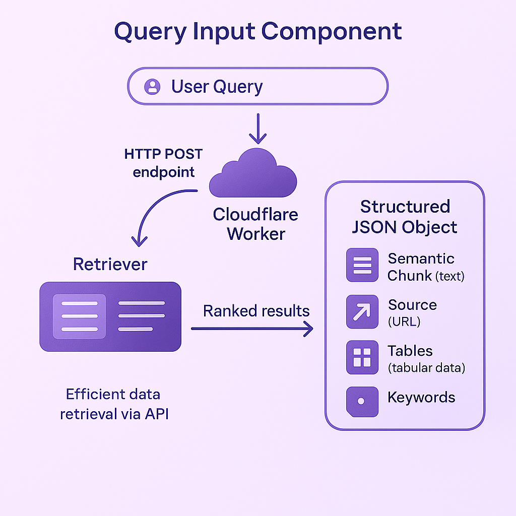
Architectural diagram of the RAG system’s query input processing pipeline
Think about how you typically interact with chatbots. User input is often not the most clear and concise, to put it mildly. However, user expectations are high. To address this, we assume by default that the input might be less than perfect, and we use the user query pipeline to process it into better-formulated queries for search. This is where prompt engineering techniques help transform raw queries into effective search parameters.
The provided input query is run through an LLM using
llama-2-13b-chat-awq hosted on Cloudflare. We use it to extract the following information from the
user query:
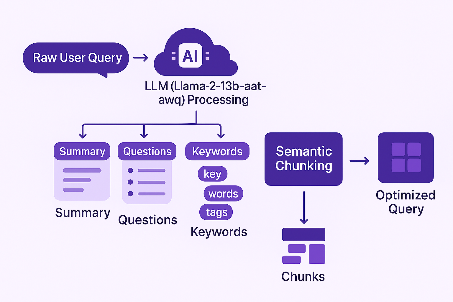
Raw user query processing pipeline and transformation flow
The output of the user query function is then sent to the semantic chunk function, where it’s broken into chunks suitable for running search queries on the data stores. Fine-tuning this process allows for more accurate keyword search and better overall performance.
The hallucination function serves a similar purpose as the user query function,
but instead of refining the user query, it enhances the input with additional
content to improve search results. We accomplish this by using an LLM
(@hf/thebloke/llama-2-13b-chat-awq
run through the Cloudflare AI
gateway) to “hallucinate” an
answer to the user query. We use the term hallucinate because the answer
generated isn’t guaranteed to be correct but provides useful additional context
for the query. This technique helps prevent inaccurate responses later in the pipeline.
For example, if the user query is “What is the capital of France?”, the hallucination pipeline might return, “The capital of France is Paris. Paris is a beautiful city with many attractions such as the Eiffel Tower and the Louvre Museum.” This extra context can improve the relevance of search results and help the semantic search process focus on the right information.
The output of the hallucination function is sent to the semantic chunk function, where it is broken into chunks suitable for running search queries on the data stores, just like in the user query pipeline.

The semantic chunk pipeline is responsible for breaking search queries into semantic chunks that can be used to run searches on the data stores. The input to the semantic chunk pipeline is a list of questions and keywords extracted by both the user query pipeline and the hallucination pipeline. Effective embedding models are crucial for this stage of retrieval augmented generation.
Unlike regular chunks, semantic chunks break down the user query based on meaning rather than token count, sentence boundaries, or arbitrary rules. This allows the search engine to better interpret the user’s intent and retrieve more relevant results. This approach to semantic search outperforms traditional keyword-based search methods for complex queries.
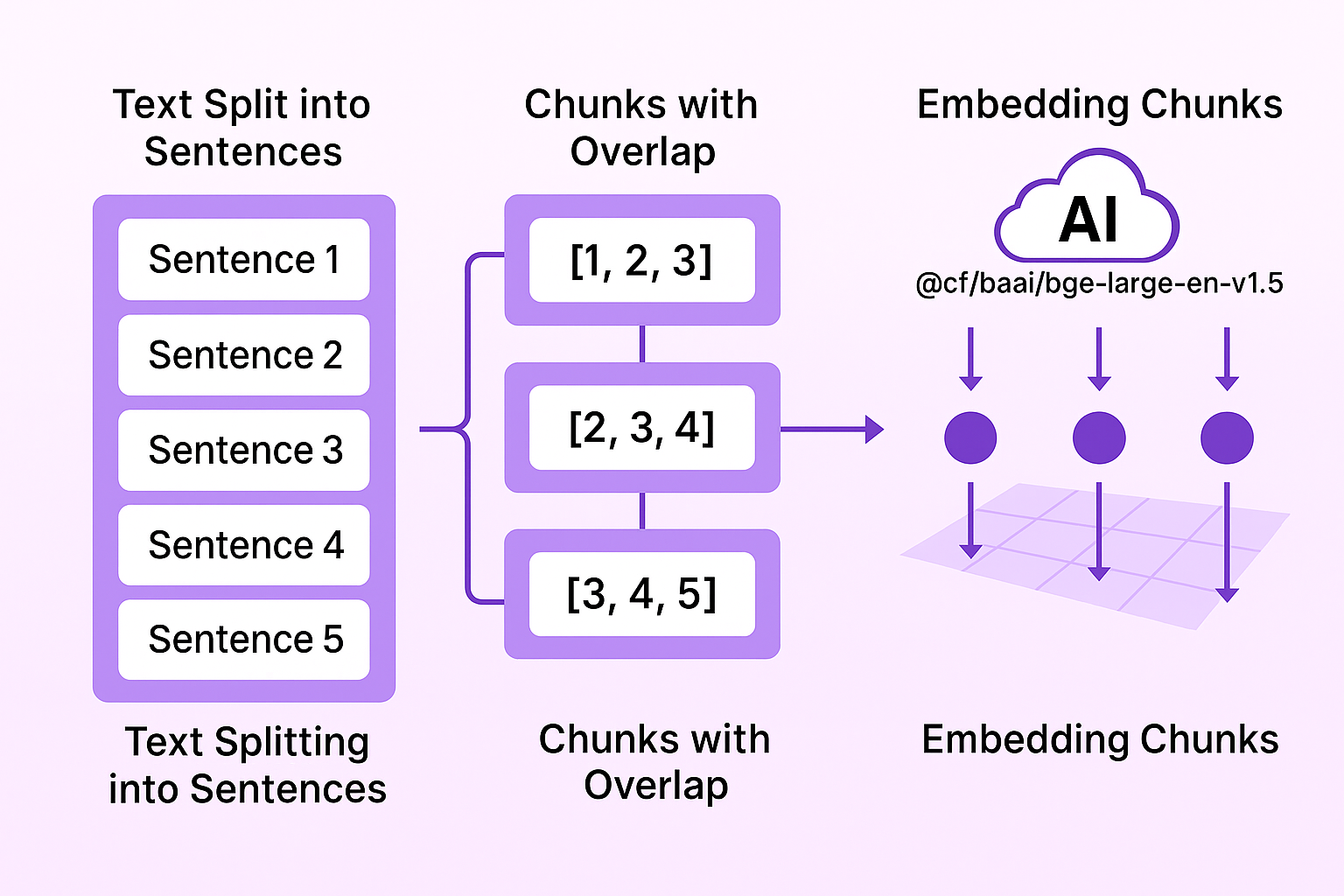
To create these semantic chunks, we first split the text into sentences and
create chunks of three sentences with a two-sentence overlap (i.e., 1,2,3,
2,3,4, 3,4,5). Each chunk is embedded using
@cf/baai/bge-large-en-v1.5
on Cloudflare. We then loop through the chunks recursively, calculating their
cosine similarity based on the vector embedding. This embedding model creates high-quality representations in the embedding space.
Cosine similarity is the cosine of the angle between the vectors; that is, it is the dot product of the vectors divided by the product of their lengths. In simpler terms, cosine similarity helps us understand how similar two vectors are. Chunks with a cosine similarity of .9 or higher are merged, unless their total length exceeds 500 tokens.
The result is a set of semantic chunks where similar concepts are merged together in chunks of no more than 500 tokens. This process is applied to all inputs, including the output from both the user query function and the hallucination function. The resulting semantic chunks are sent to the pull function to retrieve relevant data from the data stores, creating an effective hybrid search capability.
The purpose of the pull function, as the name suggests, is to pull all relevant information from various data sources. If you’ve been following our series, you know we use the following data stores:
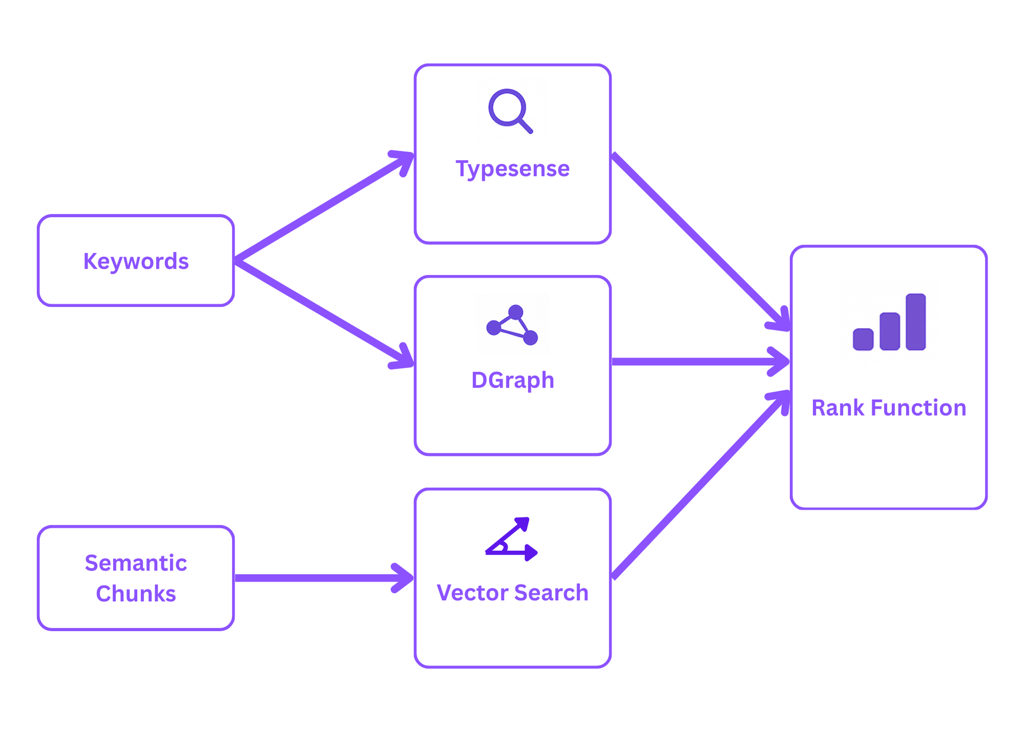
The pull pipeline takes the extracted keywords and semantic chunks to retrieve all relevant information from these multiple data sources. Specifically:
@cf/baai/bge-large-en-v1.5
to retrieve the 20 most relevant documents per semantic chunk through vector search.The result is a large amount of relevant data, which could overwhelm the context window of even the largest LLM. That’s where the rank function comes in to prioritize the most relevant data returned by the pull pipeline. This architecture helps RAG workflows access both new data and training data efficiently.
Now, you might ask: “Why don’t you just return less data?” Excellent question. While all of these techniques are designed to return relevant data, they each do so in their own way. The vector store returns the most closely related vectors (cosine similarity), the graph DB returns data about related entities, and so on. While all of this is relevant, we still need to decide which data is the most relevant. For example, if we only returned 10 items, we might end up with an order like this:
In other words, we want to return more data so the ranking algorithms can establish what’s truly relevant. Ranking algorithms can take into account context that individual data stores can’t. For instance, while the vector search works on a single chunk, the full query might contain multiple chunks. The ranking algorithm considers the entire search input, filtering through the returned results from all the stores to return the most relevant pieces.
There are several ways to rank the results from the retrieval pipeline:
Depending on your use case and available data, you might choose one or more of
these ranking methods. Since Lost Minute Travel is a demo application, we
don’t have engagement data yet, nor do we have multiple dataset versions, making
EngagementBoost and PreferOld/PreferNew unavailable for now. Because we
indexed Wikipedia, the likelihood of spammy results is low, so we can rule out
AvoidSpam. As LuckyRank is primarily for introducing diversity rather than
improving quality, we’ve decided not to use it either. That leaves us with
LLMRank and TopicRank.
Resulting in a total of 10 highly relevant documents per input query returned from the retriever pipeline, ensuring the final answer from our generative AI models has the best available source documents.

Having a human in the loop is highly beneficial when working with large language models. Even the best guardrails and ranking algorithms can’t prevent things from going off-track occasionally. This is exactly what the scoring function is designed to address. Every output from the model is tagged with a unique ID (more on that in the upcoming cognitive architecture blog). Users can provide feedback on each generated output by giving it a thumbs-up or thumbs-down.
Each thumbs up or down stores the output ID, the generated content, the input
query, and the related data points (i.e., the output from the retrieval
pipeline) in a D1 database. Over time, this builds a large dataset that can be
used for the EngagementBoost ranking algorithm, improving future outputs by
learning from previous user interactions. Additionally it provides insights into
potential blindspots in the data. This feedback loop is essential for fine-tuning the system and improving the overall quality of text generation.
Stay tuned for the next edition of this blog series where we will go into great detail about how to design a cognitive architecture for LLM prompt optimization and be sure to follow us on LinkedIn to be notified when it’s released. Schedule a free consultation with our team if you want more in-depth information on building a custom solution for SOTA RAG application using off-the-shelf components with our help, or developing a solution from scratch that leverages data analytics from code repositories and public data.
Here are answers to some of the most common questions about retrieval systems in RAG workflows:
Semantic search uses embedding models to understand the meaning behind queries, allowing the system to find content with similar meaning even when different words are used. Keyword search, on the other hand, focuses on matching specific words or phrases, which can miss relevant information if the exact terminology isn’t present. In our retrieval architecture, we use both approaches: semantic chunks with vector embeddings for meaning-based search and Typesense for keyword matching, creating a hybrid search system that maximizes relevant document retrieval.
Different types of information are best stored in different formats. Structured tabular data works well in SQL databases, relationships between entities are optimally represented in graph databases, and text is efficiently searched using vector embeddings. By using multiple data sources (D1 for SQL tables, Vectorize for embeddings, DGraph for relationships, and Typesense for text search), we can retrieve more comprehensive and accurate information, leading to better final answers from the language model.
The embedding model is crucial for translating text into vector representations that capture semantic meaning. In our retrieval system, we use @cf/baai/bge-large-en-v1.5 to create high-quality embeddings of both query chunks and stored documents. These embeddings allow us to perform vector search, finding semantically similar content in the embedding space rather than relying solely on exact text matches. The quality of these embeddings directly impacts the relevance of retrieved information.
The hallucination function uses a language model to generate additional context around the user query. While the generated content isn’t guaranteed to be factually correct (hence the term “hallucination”), it provides valuable semantic context that enriches the search query. For example, if a user asks about Paris, the hallucination function might mention the Eiffel Tower and Louvre, improving the chances of retrieving relevant documents about these landmarks even if the user didn’t explicitly mention them.
Ranking is essential because different data stores return relevant information in different ways, and we need to identify what’s most relevant to the specific query. Without ranking, even with good retrieval, the large amount of data would overwhelm the LLM’s context window and potentially dilute the quality of the generated response. Our machine learning-based ranking functions like LLMRank and TopicRank ensure that only the most relevant information influences the final answer, improving accuracy and reducing the chance of inaccurate responses.
Human feedback through our score function creates a valuable dataset for continuously improving the system. Each time users provide thumbs-up or thumbs-down reactions, we store the query, retrieved data, and generated content. This dataset helps us fine-tune ranking algorithms to prioritize content similar to what received positive feedback, identify blindspots in our data sources where the system consistently generates poor responses, and train better embedding models and search parameters based on real user interactions.
Yes, you can build an effective retrieval system using available tools and services. Our example uses Cloudflare Workers, D1, Vectorize, DGraph, and Typesense—all existing services. The implementation complexity comes from integrating these components and developing the specialized functions (user query processing, hallucination, semantic chunking, etc.) that optimize the retrieval process. While a custom solution may offer better performance for specific use cases, many organizations can achieve excellent results by thoughtfully combining existing tools with proper implementation of RAG workflows.
Handling large datasets requires a sophisticated approach beyond simple vector search. Our architecture addresses this by using multiple specialized data stores optimized for different types of data, implementing semantic chunking to break down queries effectively, employing hybrid search across multiple sources, and using machine learning-based ranking to filter the most relevant information. This layered approach allows the system to efficiently search through vast amounts of training data and new data while maintaining high relevance in returned results.
Basic RAG implementations typically use a single vector database with a straightforward similarity search. A state-of-the-art retriever elevates performance through multi-source hybrid search combining vector, keyword, and graph-based retrieval, advanced query processing with LLMs for better search parameters, sophisticated semantic chunking rather than arbitrary text splitting, machine learning-based ranking algorithms that understand context beyond individual chunks, and human feedback loops for continuous system improvement. These enhancements dramatically improve the quality and relevance of information provided to the generative AI model.